DEM Coregistration
Contents
Introduction
Coregistration of a DEM is performed when it needs to be compared to a reference, but the DEM does not align with the reference perfectly. There are many reasons for why this might be, for example: poor georeferencing, unknown coordinate system transforms or vertical datums, and instrument- or processing-induced distortion.
A main principle of all coregistration approaches is the assumption that all or parts of the portrayed terrain are unchanged between the reference and the DEM to be aligned. This stable ground can be extracted by masking out features that are assumed to be unstable. Then, the DEM to be aligned is translated, rotated and/or bent to fit the stable surfaces of the reference DEM as well as possible. In mountainous environments, unstable areas could be: glaciers, landslides, vegetation, dead-ice terrain and human structures. Unless the entire terrain is assumed to be stable, a mask layer is required.
There are multiple approaches for coregistration, and each have their own strengths and weaknesses. Below is a summary of how each method works, and when it should (and should not) be used.
Example data
Examples are given using data close to Longyearbyen on Svalbard. These can be loaded as:
import geoutils as gu
import numpy as np

import xdem
from xdem import coreg


# Load the data using xdem and geoutils (could be with rasterio and geopandas instead)
# Load a reference DEM from 2009
reference_dem = xdem.DEM(xdem.examples.get_path("longyearbyen_ref_dem"))
# Load a moderately well aligned DEM from 1990
dem_to_be_aligned = xdem.DEM(xdem.examples.get_path("longyearbyen_tba_dem")).reproject(reference_dem, silent=True)
# Load glacier outlines from 1990. This will act as the unstable ground.
glacier_outlines = gu.Vector(xdem.examples.get_path("longyearbyen_glacier_outlines"))

# Prepare the inputs for coregistration.
ref_data = reference_dem.data.squeeze()  # This is a numpy 2D array/masked_array
tba_data = dem_to_be_aligned.data.squeeze()  # This is a numpy 2D array/masked_array
# This is a boolean numpy 2D array. Note the bitwise not (~) symbol
inlier_mask = ~glacier_outlines.create_mask(reference_dem)
transform = reference_dem.transform  # This is a rio.transform.Affine object.

########################
The Coreg object
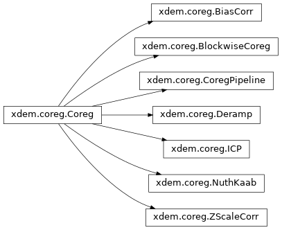
Each of the coregistration approaches in xdem inherit their interface from the Coreg class.
It is written in a style that should resemble that of scikit-learn (see their LinearRegression class for example).
Each coregistration approach has the methods:
.fit()for estimating the transform..apply()for applying the transform to a DEM..apply_pts()for applying the transform to a set of 3D points..to_matrix()to convert the transform to a 4x4 transformation matrix, if possible.
First, .fit() is called to estimate the transform, and then this transform can be used or exported using the subsequent methods.
Nuth and Kääb (2011)
Performs: translation and bias corrections.
Supports weights (soon)
Recommended for: Noisy data with low rotational differences.
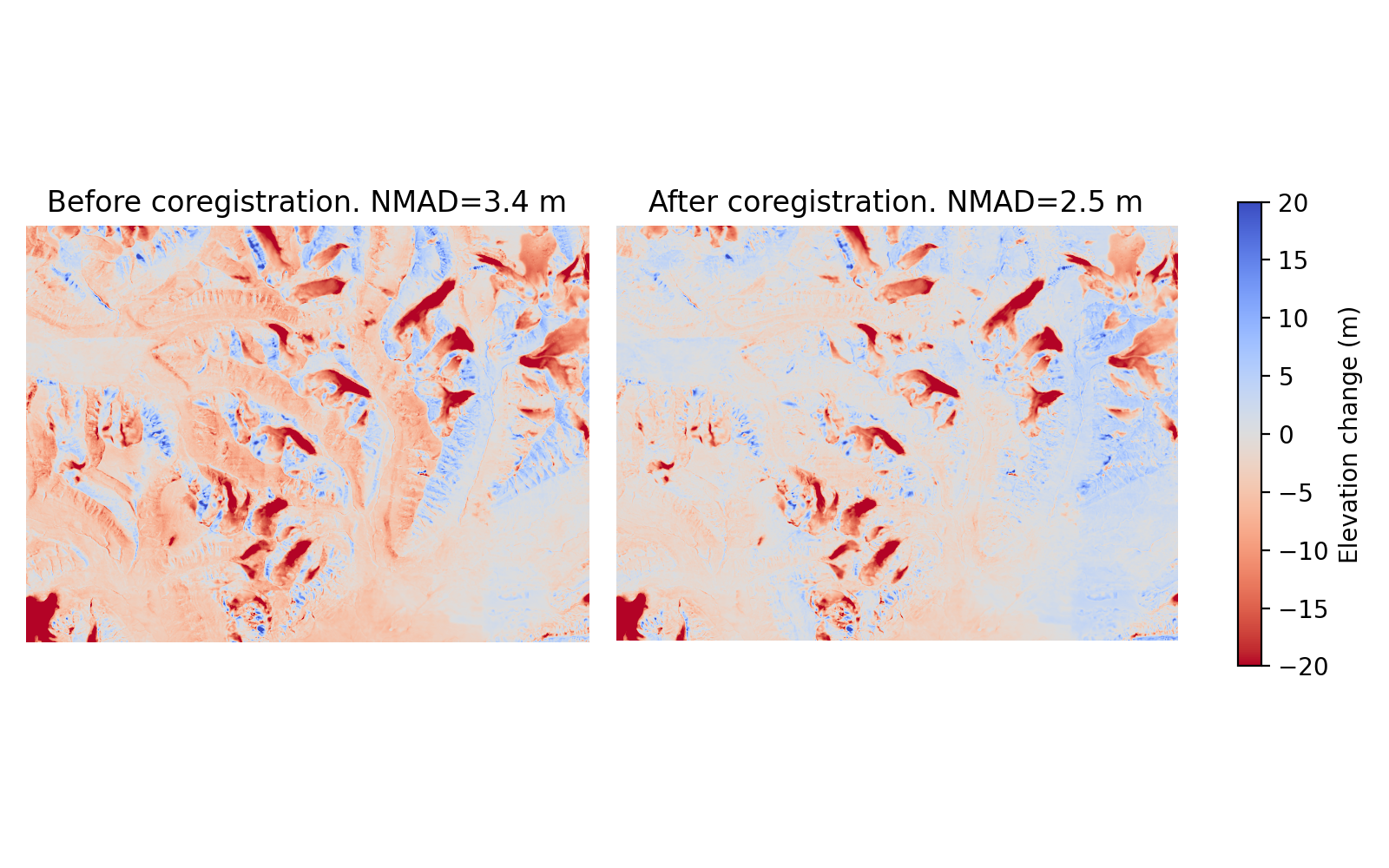
The Nuth and Kääb (2011) coregistration approach is named after the paper that first implemented it. It estimates translation and bias corrections iteratively by solving a cosine equation to model the direction at which the DEM is most likely offset. First, the DEMs are compared to get a dDEM, and slope/aspect maps are created from the reference DEM. Together, these three products contain the information about in which direction the offset is. A cosine function is solved using these products to find the most probable offset direction, and an appropriate horizontal shift is applied to fix it. This is an iterative process, and cosine functions with suggested shifts are applied in a loop, continuously refining the total offset. The loop is stopped either when the maximum iteration limit is reached, or when the NMAD between the two products stops improving significantly.
(Source code, png, hires.png, pdf)
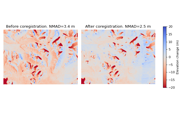
Caption: Demonstration of the Nuth and Kääb (2011) approach from Svalbard. Note that large improvements are seen, but nonlinear offsets still exist. The NMAD is calculated from the off-glacier surfaces.
Limitations
The Nuth and Kääb (2011) coregistration approach does not take rotation into account. Rotational corrections are often needed on for example satellite derived DEMs, so a complementary tool is required for a perfect fit. 1st or higher degree Deramping can be used for small rotational corrections. For large rotations, the Nuth and Kääb (2011) approach will not work properly, and ICP is recommended instead.
Deramping
Performs: Bias, linear or nonlinear height corrections.
Supports weights (soon)
Recommended for: Data with no horizontal offset and low to moderate rotational differences.
Deramping works by estimating and correcting for an N-degree polynomial over the entire dDEM between a reference and the DEM to be aligned. This may be useful for correcting small rotations in the dataset, or nonlinear errors that for example often occur in structure-from-motion derived optical DEMs (e.g. Rosnell and Honkavaara 2012; Javernick et al. 2014; Girod et al. 2017). Applying a “0 degree deramping” is equivalent to a simple bias correction, and is recommended for e.g. vertical datum corrections.
Limitations
Deramping does not account for horizontal (X/Y) shifts, and should most often be used in conjunction with other methods.
1st order deramping is not perfectly equivalent to a rotational correction: Values are simply corrected in the vertical direction, and therefore includes a horizontal scaling factor, if it would be expressed as a transformation matrix. For large rotational corrections, ICP is recommended.
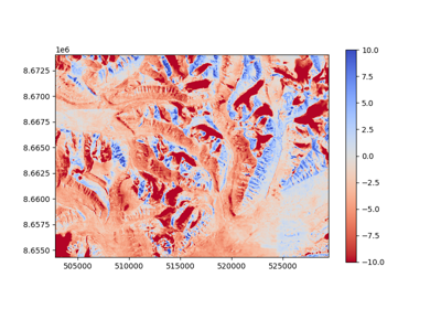
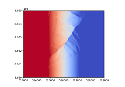
Example
# Instantiate a 1st order deramping object.
deramp = coreg.Deramp(degree=1)
# Fit the data to a suitable polynomial solution.
deramp.fit(ref_data, tba_data, transform=transform, inlier_mask=inlier_mask)

# Apply the transformation to the data (or any other data)
deramped_dem = deramp.apply(dem_to_be_aligned.data, transform=dem_to_be_aligned.transform)
Bias correction
Performs: (Weighted) bias correction using the mean, median or anything else
Supports weights (soon)
Recommended for: A precursor step to e.g. ICP.
BiasCorr has very similar functionality to Deramp(degree=0) or the z-component of Nuth and Kääb (2011).
This function is more customizable, for example allowing changing of the bias algorithm (from weighted average to e.g. median).
It should also be faster, since it is a single function call.
Limitations
Only performs vertical corrections, so it should be combined with another approach.
Example
bias_corr = coreg.BiasCorr()
# Note that the transform argument is not needed, since it is a simple vertical correction.
bias_corr.fit(ref_data, tba_data, inlier_mask=inlier_mask)

# Apply the bias to a DEM
corrected_dem = bias_corr.apply(tba_data, transform=None)  # The transform does not need to be given for bias

# Use median bias instead
bias_median = coreg.BiasCorr(bias_func=np.median)

# bias_median.fit(... # etc.
ICP
Performs: Rigid transform correction (translation + rotation).
Does not support weights
Recommended for: Data with low noise and a high relative rotation.
Iterative Closest Point (ICP) coregistration works by iteratively moving the data until it fits the reference as well as possible. The DEMs are read as point clouds; collections of points with X/Y/Z coordinates, and a nearest neighbour analysis is made between the reference and the data to be aligned. After the distances are calculated, a rigid transform is estimated to minimise them. The transform is attempted, and then distances are calculated again. If the distance is lowered, another rigid transform is estimated, and this is continued in a loop. The loop stops if it reaches the max iteration limit or if the distances do not improve significantly between iterations. The opencv implementation of ICP includes outlier removal, since extreme outliers will heavily interfere with the nearest neighbour distances. This may improve results on noisy data significantly, but care should still be taken, as the risk of landing in local minima increases.
Limitations
ICP often works poorly on noisy data. The outlier removal functionality of the opencv implementation is a step in the right direction, but it still does not compete with other coregistration approaches when the relative rotation is small. In cases of high rotation, ICP is the only approach that can account for this properly, but results may need refinement, for example with the Nuth and Kääb (2011) approach.
Due to the repeated nearest neighbour calculations, ICP is often the slowest coregistration approach out of the alternatives.
Example
# Instantiate the object with default parameters
icp = coreg.ICP()
# Fit the data to a suitable transformation.
icp.fit(ref_data, tba_data, transform=transform, inlier_mask=inlier_mask)

# Apply the transformation matrix to the data (or any other data)
aligned_dem = icp.apply(tba_data, transform=transform)
The CoregPipeline object
Often, more than one coregistration approach is necessary to obtain the best results.
For example, ICP works poorly with large initial biases, so a CoregPipeline can be constructed to perform both sequentially:
pipeline = coreg.CoregPipeline([coreg.BiasCorr(), coreg.ICP()])

# pipeline.fit(...  # etc.

# This works identically to the syntax above
pipeline2 = coreg.BiasCorr() + coreg.ICP()
The CoregPipeline object exposes the same interface as the Coreg object.
The results of a pipeline can be used in other programs by exporting the combined transformation matrix:
pipeline.to_matrix()
This class is heavily inspired by the Pipeline and make_pipeline() functionalities in scikit-learn.
Suggested pipelines
For sub-pixel accuracy, the Nuth and Kääb (2011) approach should almost always be used. The approach does not account for rotations in the dataset, however, so a combination is often necessary. For small rotations, a 1st degree deramp could be used:
coreg.NuthKaab() + coreg.Deramp(degree=1)
For larger rotations, ICP is the only reliable approach (but does not outperform in sub-pixel accuracy):
coreg.ICP() + coreg.NuthKaab()
For large biases, rotations and high amounts of noise:
coreg.BiasCorr() + coreg.ICP() + coreg.NuthKaab()