Nuth & Kääb (2011) coregistration

Nuth and Kääb (2011) coregistration allows for horizontal and vertical shifts to be estimated and corrected for. In xdem, this approach is implemented through the xdem.coreg.NuthKaab class.

For more information about the approach, see Nuth and Kääb (2011).

import geoutils as gu
import matplotlib.pyplot as plt

import xdem

Example files

reference_dem = xdem.DEM(xdem.examples.get_path("longyearbyen_ref_dem"), silent=True)
dem_to_be_aligned = xdem.DEM(xdem.examples.get_path("longyearbyen_tba_dem"), silent=True)
glacier_outlines = gu.Vector(xdem.examples.get_path("longyearbyen_glacier_outlines"))

# Create a stable ground mask (not glacierized) to mark "inlier data"
inlier_mask = ~glacier_outlines.create_mask(reference_dem)

plt_extent = [
    reference_dem.bounds.left,
    reference_dem.bounds.right,
    reference_dem.bounds.bottom,
    reference_dem.bounds.top,
]

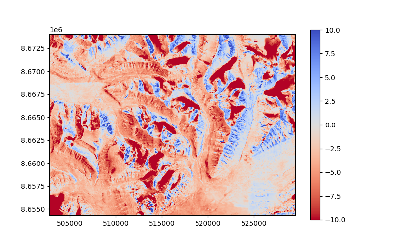
The DEM to be aligned (a 1990 photogrammetry-derived DEM) has some vertical and horizontal biases that we want to avoid. These can be visualized by plotting a change map:

diff_before = (reference_dem - dem_to_be_aligned).data

plt.figure(figsize=(8, 5))
plt.imshow(diff_before.squeeze(), cmap="coolwarm_r", vmin=-10, vmax=10, extent=plt_extent)
plt.colorbar()
plt.show()

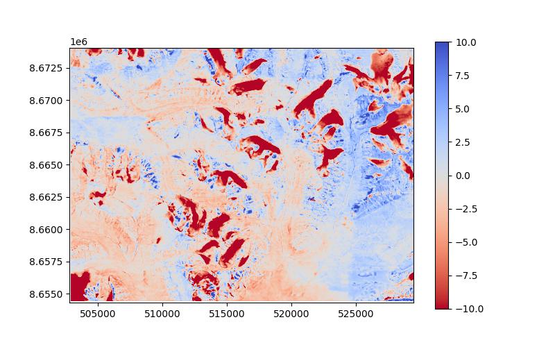
Horizontal and vertical shifts can be estimated using xdem.coreg.NuthKaab. First, the shifts are estimated, and then they can be applied to the data:

nuth_kaab = xdem.coreg.NuthKaab()

nuth_kaab.fit(reference_dem.data, dem_to_be_aligned.data, inlier_mask, transform=reference_dem.transform)

aligned_dem_data = nuth_kaab.apply(dem_to_be_aligned.data, transform=dem_to_be_aligned.transform)

Then, the new difference can be plotted to validate that it improved.

diff_after = reference_dem.data - aligned_dem_data

plt.figure(figsize=(8, 5))
plt.imshow(diff_after.squeeze(), cmap="coolwarm_r", vmin=-10, vmax=10, extent=plt_extent)
plt.colorbar()
plt.show()

We can compare the NMAD to validate numerically that there was an improvment:

print(f"Error before: {xdem.spatial_tools.nmad(diff_before):.2f} m")
print(f"Error after: {xdem.spatial_tools.nmad(diff_after):.2f} m")

Out:

Error before: 3.81 m
Error after: 2.82 m

In the plot above, one may notice a positive (blue) tendency toward the east. The 1990 DEM is a mosaic, and likely has a “seam” near there. Blockwise coregistration tackles this issue, using a nonlinear coregistration approach.