DEM subtraction and volume change
Contents
Example data
Example data in this chapter are loaded as follows:
from datetime import datetime

import geoutils as gu
import numpy as np

import xdem


# Load a reference DEM from 2009
dem_2009 = xdem.DEM(xdem.examples.get_path("longyearbyen_ref_dem"), datetime=datetime(2009, 8, 1))
# Load a DEM from 1990
dem_1990 = xdem.DEM(xdem.examples.get_path("longyearbyen_tba_dem"), datetime=datetime(1990, 8, 1))
# Load glacier outlines from 1990.
glaciers_1990 = gu.Vector(xdem.examples.get_path("longyearbyen_glacier_outlines"))
glaciers_2010 = gu.Vector(xdem.examples.get_path("longyearbyen_glacier_outlines_2010"))

# Make a dictionary of glacier outlines where the key represents the associated date.
outlines = {
    datetime(1990, 8, 1): glaciers_1990,
    datetime(2009, 8, 1): glaciers_2010,
}

# Fake a future DEM to have a time-series of three DEMs
dem_2060 = dem_2009.copy()
# Assume that all glacier values will be 30 m lower than in 2009
dem_2060.data[glaciers_2010.create_mask(dem_2060)] -= 30
dem_2060.datetime = datetime(2060, 8, 1)
Subtracting rasters
Calculating the difference of DEMs (dDEMs) is theoretically simple, but can in practice often be time consuming.
In xdem, the aim is to minimize or completely remove potential pitfalls in this analysis.
Let’s assume we have two perfectly aligned DEMs, with the same shape, extent, resolution and coordinate referencesystem (CRS) as each other. Calculating a dDEM would then be as simple as:
dem1, dem2 = dem_2009, dem_1990

ddem_data = dem1.data - dem2.data
# If we want to inherit the georeferencing information:
ddem_raster = xdem.DEM.from_array(ddem_data, dem1.transform, dem2.crs)
But in practice, our two DEMs are most often not perfectly aligned, which is why we might need a helper function for this:
xdem.spatial_tools.subtract_rasters()
ddem_raster = xdem.spatial_tools.subtract_rasters(dem1, dem2)
So what does this magical function do?
First, the nonreference; dem2, will be reprojected to fit the shape, extent, resolution and CRS of dem1.
This behaviour can be switched by changing the default reference="first" to reference="second".
Cubic spline interpolation is used by default to resample the data, which is sometimes slow, but provides the most accurate resampling results.
This can be changed with the resampling_method= keyword, for example to "bilinear" or "nearest" (see the rasterio docs for the full suite of options).
Most often, xdem works with Masked Arrays, where the mask signifies cells to exclude (presumably areas of no data).
The subtract_rasters() function makes sure that the outgoing mask is the union of the two ingoing masks.
dDEM interpolation
There are many approaches to interpolate a dDEM.
A good comparison study for glaciers is McNabb et al., (2019).
So far, xdem has three types of interpolation:
Linear spatial interpolation
Local hypsometric interpolation
Regional hypsometric interpolation
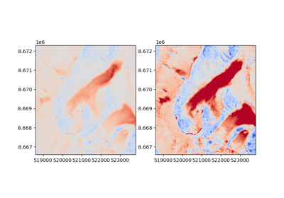
Let’s first create a xdem.ddem.dDEM object to experiment on:
ddem = xdem.dDEM(
    raster=xdem.spatial_tools.subtract_rasters(dem_2009, dem_1990),
    start_time=dem_1990.datetime,
    end_time=dem_2009.datetime
)

# The example DEMs are void-free, so let's make some random voids.
ddem.data.mask = np.zeros_like(ddem.data, dtype=bool)  # Reset the mask
# Introduce 50000 nans randomly throughout the dDEM.
ddem.data.mask.ravel()[np.random.choice(ddem.data.size, 50000, replace=False)] = True
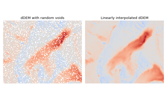
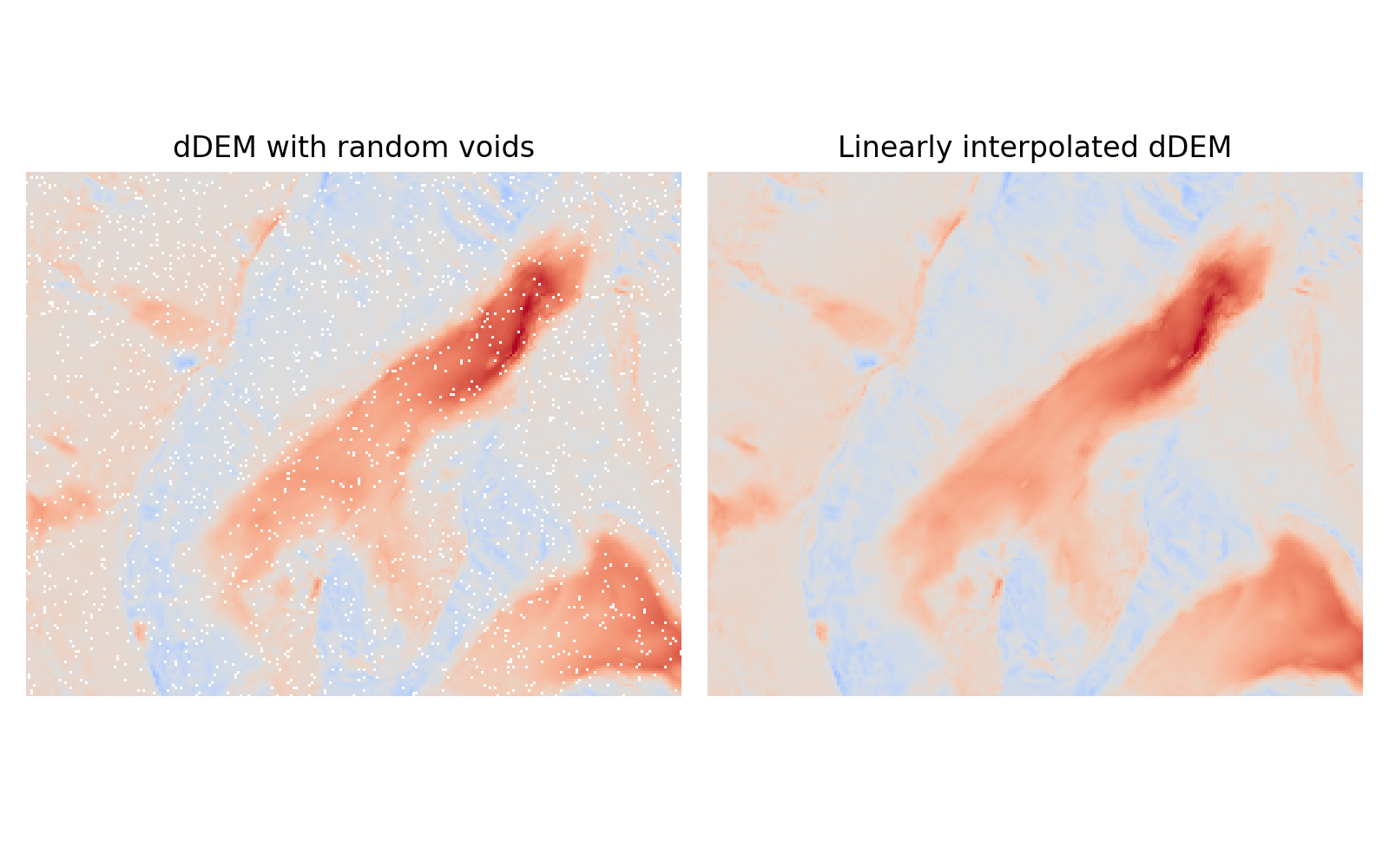
Linear spatial interpolation
Linear spatial interpolation (also often called bilinear interpolation) of dDEMs is arguably the simplest approach: voids are filled by a an average of the surrounding pixels values, weighted by their distance to the void pixel.
ddem.interpolate(method="linear")
(Source code, png, hires.png, pdf)
Local hypsometric interpolation
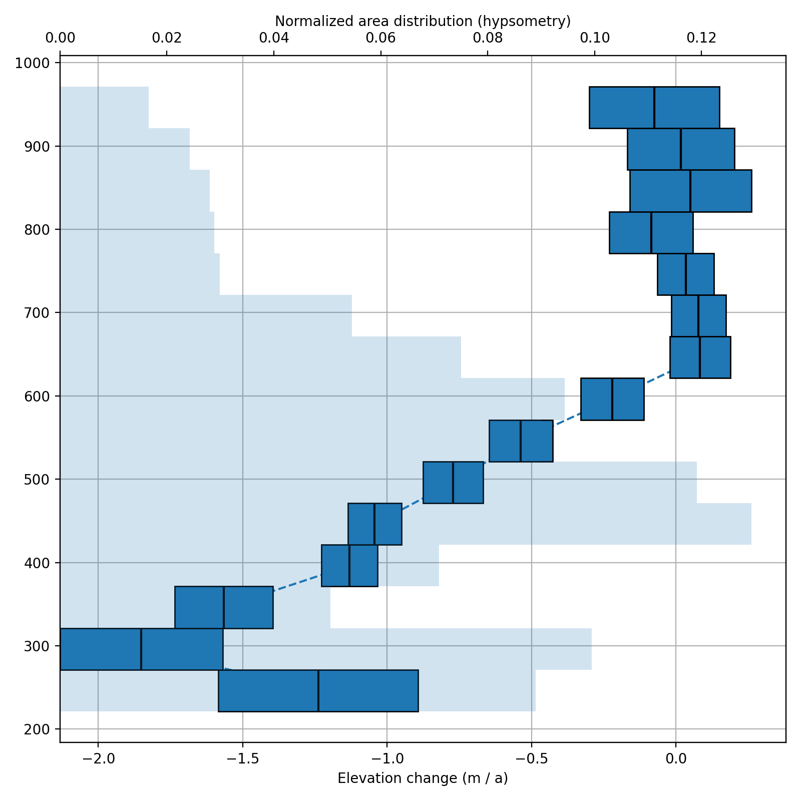
This approach assumes that there is a relationship between the elevation and the elevation change in the dDEM, which is often the case for glaciers. Elevation change gradients in late 1900s and 2000s on glaciers often have the signature of large melt in the lower parts, while the upper parts might be less negative, or even positive. This relationship is strongly correlated for a specific glacier, and weakly correlated on regional scales (see Regional hypsometric interpolation). With the local (glacier specific) hypsometric approach, elevation change gradients are estimated for each glacier separately. This is simply a linear or polynomial model estimated with the dDEM and a reference DEM. Then, voids are interpolated by replacing them with what “should be there” at that elevation, according to the model.
ddem.interpolate(method="local_hypsometric", reference_elevation=dem_2009, mask=glaciers_1990)
(Source code, png, hires.png, pdf)
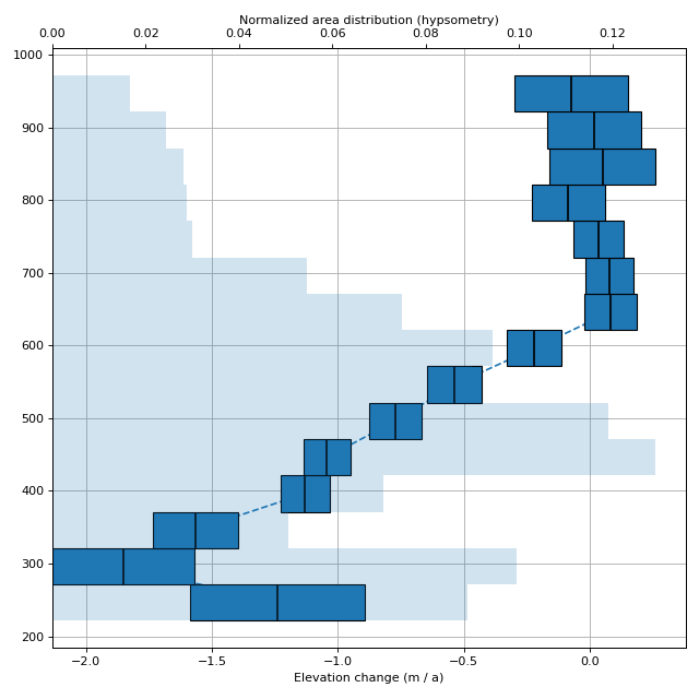
Caption: The elevation dependent elevation change of Scott Turnerbreen on Svalbard from 1990–2009. The width of the bars indicate the standard devation of the bin. The light blue background bars show the area distribution with elevation.
Regional hypsometric interpolation
Similarly to Local hypsometric interpolation, the elevation change is assumed to be largely elevation-dependent. With the regional approach (often also called “global”), elevation change gradients are estimated for all glaciers in an entire region, instead of estimating one by one. This is advantageous in respect to areas where voids are frequent, as not even a single dDEM value has to exist on a glacier in order to reconstruct it. Of course, the accuracy of such an averaging is much lower than if the local hypsometric approach is used (assuming it is possible).
ddem.interpolate(method="regional_hypsometric", reference_elevation=dem_2009, mask=glaciers_1990)
(Source code, png, hires.png, pdf)
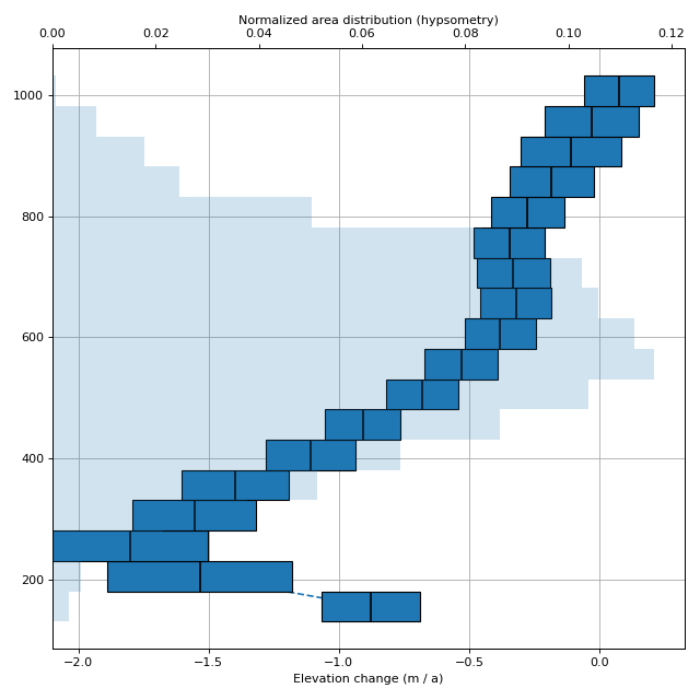
Caption: The regional elevation dependent elevation change in central Svalbard from 1990–2009. The width of the bars indicate the standard devation of the bin. The light blue background bars show the area distribution with elevation.
The DEMCollection object
Keeping track of multiple DEMs can be difficult when many different extents, resolutions and CRSs are involved, and xdem.demcollection.DEMCollection is xdem’s answer to make this simple.
We need metadata on the timing of these products.
The DEMs can be provided with the datetime= argument upon instantiation, or the attribute could be set later.
Multiple outlines are provided as a dictionary in the shape of {datetime: outline}.